3часть1308.2705Stochastic Models Predict User Behavior_3чел. Закон серфинга p 14 6 л 14 8
 Скачать 74.28 Kb. Скачать 74.28 Kb.
|

|
^Tespond (u) (14) параметр value закон серфинга p =14 ± 0.6 Л = 14 ± 1.8 просмотров за сообщение v = 38 ± 20 ответ заинтересованным сторонником Pact = 0.12 ± 0.03 ТАБЛИЦА III Параметры модели, оценённые по данным события @YESONPROP30.
Мы оцениваем значения параметров модели по максимуму правдоподобия: выбор параметров модели, которые максимизируют вероятность наблюдаемых ответов от набора пользователей в соответствии с моделью. Мы рассматриваем пользователей как отвечающих независимо друг от друга, поэтому вероятность наблюдаемых ответов является результатом Prespond (u) для каждого пользователя, из уравнения. 11. Для этой максимизации нам нужны только факторы, зависящие от параметров модели, т. е. значение А, входящее в уравнение 12. Все остальные значения известны из пользовательских данных. Для удобства мы берём логарифм этого выражения, тем самым максимизируя ^ log(L(u)) (13) u где сумма превышает всех пользователей u в обучающем наборе, которые мы принимаем за последователей @ YesOnProp30. Последователи остальных адвокатов, перечисленные в таблице I, являются нашим набором тестов для оценки модели. Наша модель не определяет закон параметров серфинга сверх требования, чтобы p «A максимизировало вероятность. Это связано с тем, что вероятность почти одинакова, если пользователи дважды посещают Twitter дважды, но только смотрят на половину количества элементов в своем списке, т. Е. Масштабируют v ^ 2v при делении p и A на 2. Таким образом, для этого исследования мы используем закон параметров серфинга, определенный для предварительного изучения социальных сетей [5], умножая на 15 для преобразования из «номера страницы» в «номер позиции» в списке новых сообщений. Эти параметры имеют p «A, поэтому согласуются с нашей моделью для Twitter. В таблице III приведены оценки максимального правдоподобия параметров модели с диапазонами, указывающими доверительные интервалы в 95%. IV. Результаты Мы оцениваем модель на тестовом наборе, состоящем из последователей второго-четвертого адвокатов в таблице I. Таким образом, мы используем параметры модели, оцененные для одного защитника (@ YesOnProp30), чтобы предсказать поведение последователя для трех других адвокатов. Мы сравниваем предсказания стохастической модели с базовой моделью регрессии, которая описывается далее.
Для сравнения со стохастической моделью мы рассматриваем модель логистической регрессии, связывающую общую активность пользователя с ответом на должности адвокатов. в отличие от стохастической модели, регрессионная модель не рассматривает пользователя как переход через ряд состояний для принятия решения об ответе. Вместо этогоsimply considers users who are more active on the site are also more likely to respond. Since user activity varies over a wide range and has a long tail, we find a regression on the log of the activity rate, i.e., log Rposts(u), provides better discrimination of response than a using Rposts itself. Determining the fit based on the same training set as used with the stochastic model, i.e., the followers of @YesOnProp30, we find 1 1 + exp(-(во + в1 log(Rposts(u)))) with в0 = -5.01 ± 0.06 and в1 =0.11 ± 0.03.
For testing, the actual response M is the dependent variable predicted by the model. Specifically, the model gives the distribution of M for a user (Eq. 11) based on the model parameters (Table III), and other data for that user (i.e., the values in Table II other than M). We use the expected value from this distribution as the model’s prediction of M. model
TABLE IV Spearman rank correlation between model prediction and OBSERVED FOLLOWER RESPONSE. LAST COLUMN IS p-VALUE OF Spearman rank test for whether the two models have the same CORRELATION. ASTERISKS INDICATE CORRELATIONS NOT SIGNIFICANTLY DIFFERENT FROM ZERO AT 5% p-VALUE BY SPEARMAN RANK TEST. Table IV shows the Spearman rank correlation between the predicted and observed number of responses for users in each test set. Note that the first line reports results of testing on the data used for training the model. The last column reports the p-value of a statistical test to identify differences between the models. The closer this value is to zero, the more confidence this gives for rejecting the hypothesis that the two models actually have the same correlation and just produced the observed difference in correlation on these samples of users by chance. Overall, the stochastic model has a larger correlation except for @StopProp30, where the relatively small number of followers and advocate posts (see Table I) are not sufficient to identify differences from the regression model. The model provides a distribution of responses, not just a single prediction. This additional information from the model is an indication of the accuracy of the prediction. Table V shows one characterization of this accuracy: the Spearman rank correlation between prediction error and the standard deviation of the distribution returned by the model. The prediction error is the absolute value of the difference between the expected value of the distribution and the observed number of responses to the advocate posts. The stochastic model has a larger correlation except for @StopProp30. Correlations are larger than those of the prediction itself (Table IV). Wefind that while variability of user behavior not included in the model gives many relatively large prediction errors, the standard deviation of the model nevertheless provides a good ranking of the prediction accuracy. model
TABLE V Spearman rank correlation between prediction error and STANDARD DEVIATION OF MODEL DISTRIBUTION. The Spearman rank correlation values for training and testing the model on the same population of users (@YesOn- Prop30) is similar to the correlation values when training on one population (@YesOnProp30) and testing on the other populations (@StopProp30, @CARightToKnow,@NoProp37). This highlights the power of stochastic models to learn from one campaign and transfer to another, despite differences between individual campaigns, including those due to the issues involved, campaigner style, follower preferences, etc.
In addition to using the model to predict how many advocate posts a user will respond to, models can classify users by their relative response among all the advocate's followers. For instance, models can identify the subset of users who are likely to respond the most to advocate posts rather than precisely predicting how often they will respond. This classification of users is analogous to classifying content on social media sites, e.g., distinguishing stories likely to get many or few votes rather than predicting the precise number of votes [5]. Such predictions form the basis of using crowd sourcing to select a subset of submitted content to highlight [22]. As an example, we apply the stochastic model to predict which users in the test set will be among the top 25% of responders, measured by the fraction of advocate posts they responded to. One way to use a model for this classification task is to select the users whose predicted response is among the top 25% of those predictions. Model performance on this classification task is then the extent these selected users correspond to the actual top responders. Table VI shows the fraction of users in the test set incorrectly classified by this procedure, i.e., the fraction of users predicted to be among the top 25% who were not, or vice versa. The table also shows the precision and recall of this classification, i.e., fractions of predicted top responders who are, and fraction of top responders who are predicted to be so, respectively. In this case, classification by the stochastic model is significantly better than a random classifier, i.e., randomly selecting 25% of the users. On the other hand, the regression model is consistent with random classification. A more general measure of classification performance is the precision vs. recall curve, shown in Fig. 6. For each model, model error fraction precision recall random? stochastic 30% 40% 40% 10-4 regression 36% 27% 27% 0.2 TABLE VI Classification of top 25% responders. The last column is the p-VALUE OF THIS ERROR RATE ARISING FROM A RANDOM CLASSIFIER ACCORDING TO THE FISHER EXACT TEST OF PROPORTIONS [23] find top 25% responders out of 351 (test set) 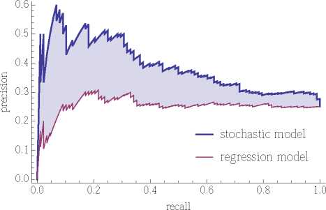 Fig. 6. Precision vs. recall for identifying top responders. we sort the U = 351 users in the test set according to their predicted fraction of response to the advocate's posts. For k = 1,... ,U, we examine the set of users with the k largest predicted responses. For example, when k = 1 the set is the single user with the largest predicted response, and when k = U the set has all users. As k increases, the figure shows the fraction of these k users that are among the observed top 25% responders (precision) vs. the fraction of the observed top responders included among the k users (recall). Better classifiers have higher curves in this figure: able to identify a large fraction of the actual top responders without also including many less responsive users. By comparison, random selection of users would give, on average, 25% precision for any value of recall. The curve for the regression model does not differ significantly from this precision value. A specific classifier using this procedure amounts to se lecting a position on the precision-recall curve by picking the number of users to consider as the top responders, i.e., a value of k. For instance, the values in Table VI correspond to k = 88, i.e., 25% of the 351 users in the test set. In practice, selecting a position on the curve, i.e., choice of k, depends on how important it is to avoid false positives vs. false negatives. In the example discussed in Fig. 6, with somewhat smaller values of k, the stochastic model gives higher precision.
Both stochastic models and simpler regression models can classify users based on their likely response. However, the stochastic model can also estimate underlying state transition probabilities for users. For instance, this could distinguish users who do not respond mainly due to visibility (e.g., users who follow many others or do not visit Twitter often) from those who do not respond due to lack of interest. The former group, i.e., interested users who do not see the advocate posts, would be more likely to respond to higher-visibility messages (e.g., direct mail) than the latter group. Thus this classification based on why users are not responding could help the advocate focus limited resources on reaching supportive users. Since the model characterizes user interest by a distribution of values, the model can not only suggest users with high interest but also estimate the confidence in that assessment based on the width of the distribution. As an example, Fig. 7 shows how the visibility-adjusted prediction alters the estimated likely range of user interest after observing how that user responds. The prior distribution (Eq. 8), before observing responses to advocate posts, is from a content analysis of the user’s posts. For the user in Fig. 7(a), the values are m = 3 and n = 5, which suggests a relatively high interest in the topic, but with large uncertainty due to the small number of posts by that user. After observing the user responses to advocate posts (in this case, responding to M = 3 of N = 391 posts), the posterior distribution for Ptopic is proportional to the integrand of Eq. 11. This combines the prior distribution with response due to a combination of visibility and interest to give the posterior distribution of Ptopic shown in the figure. In this case, the posterior distribution suggests a user with relatively low interest. By contrast, Fig. 7(b) shows the estimates for an apparently similar user: m = 5 and n = 7 and responding to only M = 2 out of N = 391 advocate posts. In this case, the model accounts for the low response as due to low visibility of the advocate’s posts and estimates the user’s interest in the topic is likely a bit higher than expected from the prior content analysis of the user’s posts. Thus, according to the model, this user is likely far more interested in the topic than suggested by the low response to advocate posts. To test the predicted difference in interest between these users, we examined additional data on their posts. The first user is a news reporter from outside California who fol lows only one advocate, namely @NoProp37, and focuses on national politics rather than California state politics. The second user follows 25 advocates, including 10 who post on proposition 37, on both sides of the issue. Thus the second user appears significantly more interested in the topic than the first, consistent with the model prediction shown in Fig. 7.
We find that both prediction of response and classification are better when we account for transitions among user states involved in social media than using a statistical regression based on overall activity. In particular, even with crude estima tion of the model properties, using the state-based model leads to better predictions. In practice, data from social media often do not include all relevant details of user behavior (e.g., when they visit the site or view particular content). Thus, this study shows stochastic models can give reasonable performance in practice despite using coarse estimates based only on readily observed behavioral data. However, the relatively low absolute performance for the stochastic model shows that user-specific details not accounted for are important for improving accuracy. For instance, the rate of receiving new posts depends on the activity rate of a user’s friends, Pposts(friends(M)), which we approximated by Pposts, the typical posting rate within a population of users. The distribution of user activity varies considerably, having a long tail. Some users are quite prolific, while others rarely post. Thus data on the activity of each user’s friends could improve the model by providing Pposts on a user-specific basis. Another model parameter, Pact(u), estimates a user’s likeli hood to retweet interesting advocate posts. We took this value to be the average over all users, Pact. However, people use retweets differently. Some users mainly retweet posts rather than posting original material, indicating a higher probability of responding to a viewed tweet. Other users have almost no retweets, suggesting these users prefer not to rebroadcast posts. This user-specific variation could contribute to the difference between the prior and posterior distribution seen in Fig. 7. A possible extension of our model is to use each user’s propensity to retweet in general as part of estimating Pact(u) for that user. Not every post by an advocate is of interest to all of the followers, such as a post directed to another user. Therefore, a user’s interest in a tweet depends on the post’s appeal and the individual’s interest in the topic. A direction for future work is to use the overall response to the tweet as an indication of its appeal. The model would then combine both the user’s estimated topic interest and the community’s overall interest in each tweet to determine the user’s interest in that particular tweet. By addressing the tweet-specific interest, this could improve Pact by including a measure of the content, i.e., the appeal of a post, instead of assuming all advocate posts are equally appealing, on average. This contrasts with the improvement to Pact mentioned above, which focuses on differences in a user’s tendency to respond in general. V. Related Work Stochastic models are the basis of population dynamics models used in a variety of fields, including statistical physics, demographics, epidemiology, and macroeconomics. In the context of social media, stochastic models identify mecha nisms relating the design of social media sites to the behavioral outcomes of their users. Previous applications of the stochastic modeling framework focused on describing the aggregate behavior of many people by average quantities [11], [12], [6], such as the average rates at which people contribute content or respond to emails, and so on. A series of papers applied the stochastic modeling framework to social media, specifically to examine the evolution of popularity of individual items shared on the social news aggregator Digg [9], [10], [5], [6]. These studies assumed the user population had similar interest in each item, or similar when separated in broad populations (e.g., follower or not of the item’s submitter), whereas the quality of each shared news item varied, leading to differences in their eventual popularity. In this paper, by contrast, we 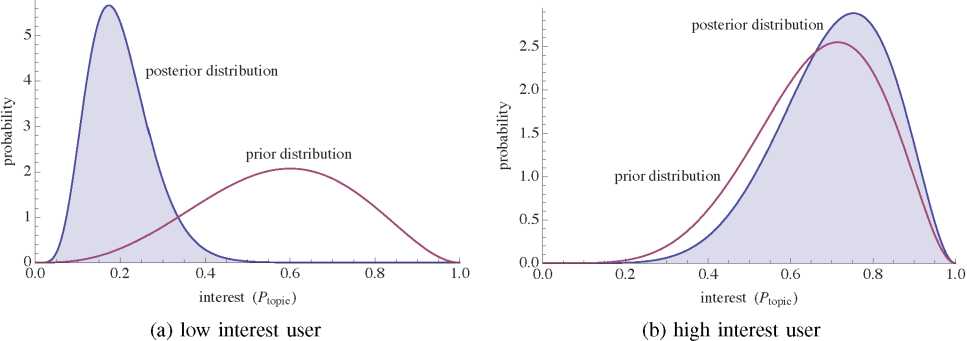 Fig. 7. Estimated prior distribution of Ptopic values for two users and posterior distribution after observing how the users respond to advocate posts. (a) Low interest user with 3 out of 5 posts on topic, who responds to 3 of 391 advocate posts. (b) High interest user with 5 out of 7 posts on topic, who responds to 2 of 391 advocate posts. apply the models to describe and predict the behavior of an individual user, averaging over any differences in quality of content (i.e., the advocate’s posts). When inferring response of users to items shared on social media, computer scientists generally consider only user’s interest in the topics of an item [1], [3], [4], or the number of friends who have previously shared the item [24]. However, as we have demonstrated in this paper, response is conditioned on both interest and visibility of the item, so that a lack of response should not indicate a lack of interest. Failing to account for the visibility of items can lead to erroneous estimates of interest and influence [25]. Stochastic modeling framework allows us to factor in the visibility of items in a principled way. Stochastic models are similar to Hidden Markov Models (HMMs) frequently used to model systems in which the ob served behavior of an individual is a result of some unobserved (or hidden) states (see, e.g., [26]). In contrast to HMMs, the goal of which is to identify hidden states that maximize the probability of an observed action sequence, stochastic models are best suited for predicting the evolution of the ob served actions of a population of individuals. Population-level analysis, combined with relevant independence assumptions, enables stochastic models to parsimoniously describe observed behavior of many individuals, and also leads to more tractable parameter inference. VI. Conclusion We showed that a stochastic model of user behavior gives useful predictions even when available data does not include aspects of user behavior most relevant for estimating model parameters. Instead, we used readily available proxy estimates. We attribute success of the stochastic modeling approach to capturing relevant details of user behavior in social media that, although unobserved, condition the observed behavior. Perhaps the most important aspect of behavior our stochastic model accounts for is visibility of the post, which depends on how many newer posts are above it on the user’s list,and how likely the user is to scan through at least that many posts. We demonstrated that accounting for visibility allows us to more accurately predict response and determine a user’s actual interest in the topic. We see performance gains even with simple parameter estimates based on population wide averages, suggesting the possibility that a model that better accounts for user heterogeneity will produce even better quantitative insights. The applications highlighted in this paper do not exhaust the list of potential applications of stochastic models. Addi tional applications include predicting response to new posts from early user reactions (e.g., as with Digg [5]), and using visibility-adjusted response to determine most useful or compelling campaign messages to show to new users (i.e., a “visibility-adjusted” popularity measure). our treatment considers user parameters as static. However, user’s activity, interest in the topic and willingness to support the advocate could change in time. The stochastic model could incorporate changes by re-estimating parameters over time. This could provide useful feedback to the advocate to gauge reaction to specific campaigns. In particular, by separating out the effects of visibility, the model could indicate how the level of interest changes after the campaign. Acknowledgements We thank Suradej Intagorn for collecting the data used in this study. This material is based upon work supported in part by the Air Force Office of Scientific Research under Contract Nos. FA9550-10-1-0569, by the Air Force Research Labo ratories under contract FA8750-12-2-0186, by the National Science Foundation under Grant No. CIF-1217605, and by DARPA under Contract No. W911NF-12-1-0034. References
|